Nürnberg - 1. Viewshed Greenness Visibility Index (VGVI)

Introduction

The visibility of greenspace is crucial for understanding how urban environments influence mental health and well-being. In contrast to simple 2D buffer analyses, visibility focuses on the eye-level perspective: how much greenery a person sees from their usual vantage point. One way to estimate this is by using street-view (SV) images (e.g., from Google Street View or Baidu Street View). However, SV-based methods are often limited by seasonal inconsistencies and coverage gaps on roads inaccessible by car (Li et al. 2015). A promising alternative is viewshed analysis within a GIS framework, which can accurately simulate what a person can see from specific locations. Recent studies at city-wide scales show this approach yields highly accurate visibility estimates, without depending on SV image availability (Tabrizian et al. 2020; Labib, Huck, and Lindley 2021; Cimburova and Blumentrath 2022). Improved computation times now allow large-scale assessments of visible greenspace with relatively little effort (Brinkmann, Kremer, and Walker 2022). This measure of greenspace visibility is especially relevant for the restoration pathway, where greenery supports mental recovery (Markevych et al. 2017).

Ample evidence suggests that exposure to green spaces can significantly lower stress and restore cognitive function. According to the stress reduction theory, natural environments promote stress relief by providing visual cues perceived as safe havens in evolutionary terms (Ulrich 1981; Ulrich et al. 1991). Meanwhile, the attention restoration theory posits that nature helps the mind recover from “attention fatigue” by engaging involuntary attention, thus giving directed attention a chance to rest (Kaplan and Kaplan 1989). Both theories underscore the importance of simply seeing natural elements for psychological benefits. As a result, the inclusion of visibility metrics - from either street-view imagery or GIS-based viewshed analysis - can add vital insights into how greenspace fosters restoration and supports better mental health outcomes (Dadvand et al. 2016).

Data

The relevant spatial datasets have been uploaded on Zenodo: administrative boundaries (AOI), DTM and DSM rasters, and a binary land-cover raster for greenspace analysis. All raster data is available at 1m resolution.

library(sf)
library(dplyr)
library(terra)
library(CGEI)

zenodo_url <- "https://zenodo.org/records/14633167/files/"
# AOI
aoi <- read_sf(paste0(zenodo_url, "01_Nbg_Bezirke.gpkg")) %>%
  filter(code_bez != "97") %>% # This is not available in the GAVI
  group_by(code_bez, name_bez) %>%
  summarise() %>%
  ungroup()

# DSM
dsm <- rast(paste0(zenodo_url, "03_dsm_1m.tif"))

# DTM
dtm <- rast(paste0(zenodo_url, "03_dtm_1m.tif"))

# Greenspace (binary)
lulc <- rast(paste0(zenodo_url, "03_ndvi_01_1m.tif"))

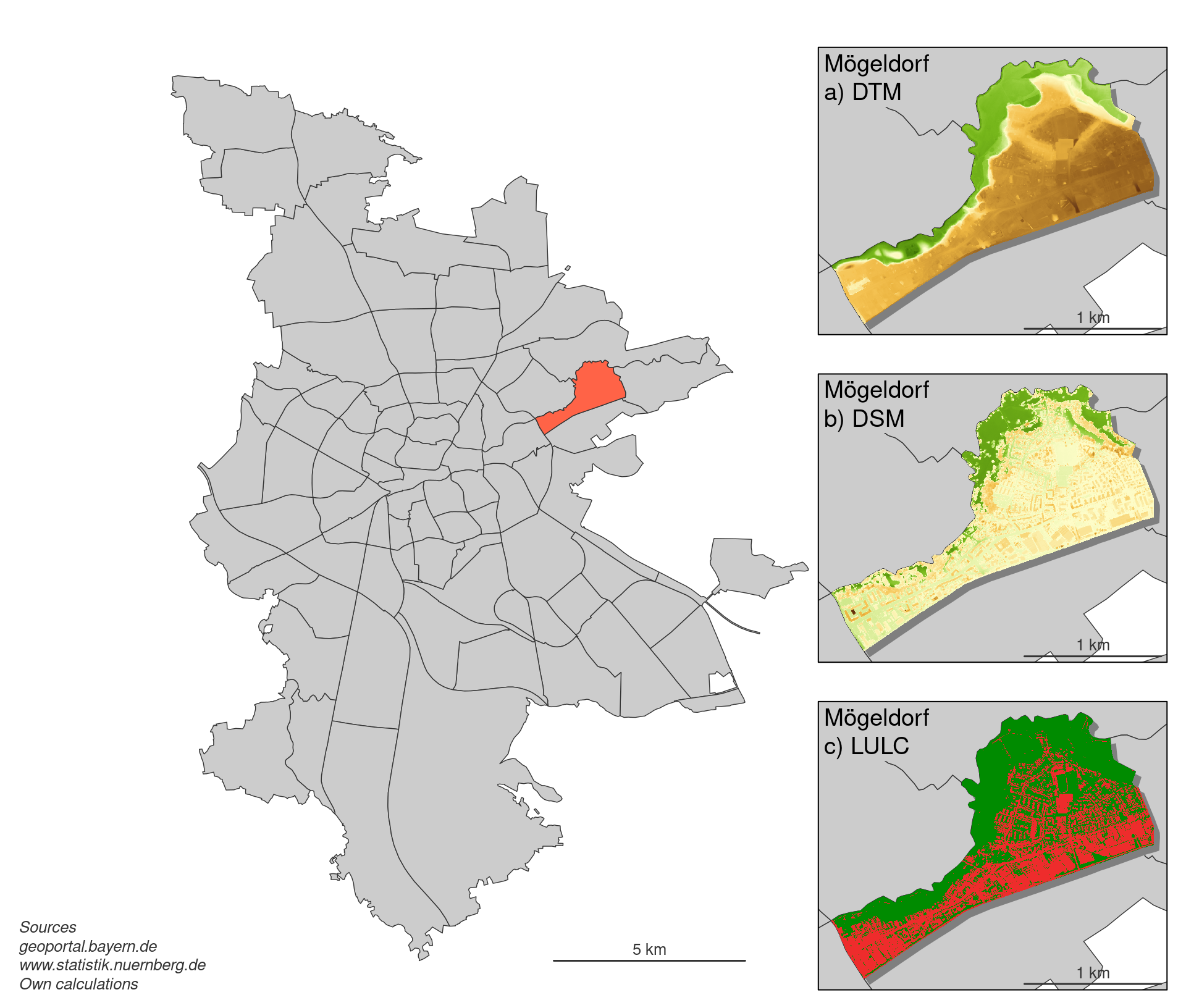
Nürnberg, shown on the left in grey, is divided into 86 administrative districts. Mögeldorf has been highlighted in orange to provide examples of the three key greenness metrics on the right:

1. DTM - The Digital Terrain Model illustrates the bare earth’s surface elevation, excluding buildings and vegetation. In the map, higher terrain is depicted in brownish colors, transitioning to green in lower-lying areas.

2. DSM - The Digital Surface Model includes all features above ground (e.g., buildings, trees). The green and yellow shades indicate varying heights, reflecting how built-up areas and vegetation rise above the terrain.

3. LULC - The land-use/land-cover map distinguishes vegetated (green) from non-vegetated (red) areas, making it easy to spot where greenery dominates versus dense urban structures.

VGVI

A key measure of eye-level greenspace exposure is the Viewshed Greenness Visibility Index (VGVI) (Labib, Huck, and Lindley 2021). This metric quantifies how much greenery (based on a binary LULC layer) is visible from a given point when accounting for local surface elevations (DSM) and terrain elevations (DTM).

1. Defining Observer Locations

To simulate where an individual might stand, we first identify valid observer points at a 5 m resolution, excluding areas where buildings or other tall structures exceed the observer’s eye height (e.g., 2.2 m above ground). The code below shows how we aggregate DSM and DTM to 5 m, filter for valid points (dsm5 <= dtm5 + 2.2), and convert these locations into an SF object:

# First we need all valid cells in a 5x5m grid. These are where the DSM is not
# higher than 1.8m + DTM
dsm5 <- aggregate(dsm, 5)
dtm5 <- aggregate(dtm, 5)

obs <- dsm5 <= (dtm5 + 2.2)
obs <- obs %>%
  crop(aoi) %>%
  mask(aoi)

obs_vals <- values(obs)
obs_vals <- which(as.vector(obs_vals))

# Convert the cell coordinates as an SF
obs_sf <- terra::xyFromCell(obs, obs_vals)
obs_sf <- st_as_sf(as_tibble(obs_sf), coords = c("x", "y"), crs = crs(dsm)) %>%
  mutate(id = 1:n()) %>%
  relocate(id)

2. Calculating the VGVI

With all potential observer locations defined, we compute the VGVI using a viewshed approach. In brief:

• The observer’s eye height (2.2 m) is placed atop the DTM, and any obstacles (e.g., buildings, trees) in the DSM are considered.

• Each visible line-of-sight cell in a viewshed is checked against the binary greenspace raster (LULC).

• A distance decay function reduces the weight of objects further away (e.g., exponential with m=1m and b=3).

Below is the vgvi() function call from the CGEI R package that performs these steps in parallel:

# Calculate VGVI
vgvi_sf <- vgvi(observer = obs_sf,
                dsm_rast = dsm, dtm_rast = dtm, greenspace_rast = lulc,
                max_distance = 500, observer_height = 2.2, 
                m = 1, b = 3, mode = "exponential",
                cores = 22, progress = TRUE)

3. Interpolating VGVI to a Continuous Surface

Finally, the point-based VGVI results (one value per observer location) are interpolated to a continuous 10 m resolution raster using Inverse Distance Weighting (IDW). IDW assumes nearby values are more similar than distant ones, so each unknown cell’s VGVI is a distance-weighted average of its nearest neighbors (Hartmann, Krois, and Waske 2018). Relevant parameters (e.g., number of neighbors, distance threshold) can be fine-tuned based on sensitivity analysis.

# Now rasterize the VGVI
vgvi_sf <- vgvi_sf[aoi,]
vgvi_rast_05 <- sf_interpolat_IDW(observer = vgvi_sf,
                                  v = "VGVI",
                                  aoi = aoi,
                                  raster_res = 5,
                                  n = 10, beta = 2, max_distance = 500,
                                  na_only = TRUE,
                                  cores = 22, progress = TRUE)

# Bring to 10m resolution
vgvi_rast_10 <- aggregate(vgvi_rast_05, 2)
vgvi_rast_10 <- vgvi_rast_10 %>%
  crop(aoi) %>%
  mask(aoi)

Finally, the VGVI raster can be classified using Jenks natural breaks to highlight different visibility classes.

# Classify the VGVI using Jenks natural breaks - N=9
vgvi_rast_10 <- CGEI:::reclassify_jenks(vgvi_rast_10, 9)
vgvi_rast_10 <- as.int(vgvi_rast_10)
names(vgvi_rast_10) <- "VGVI"

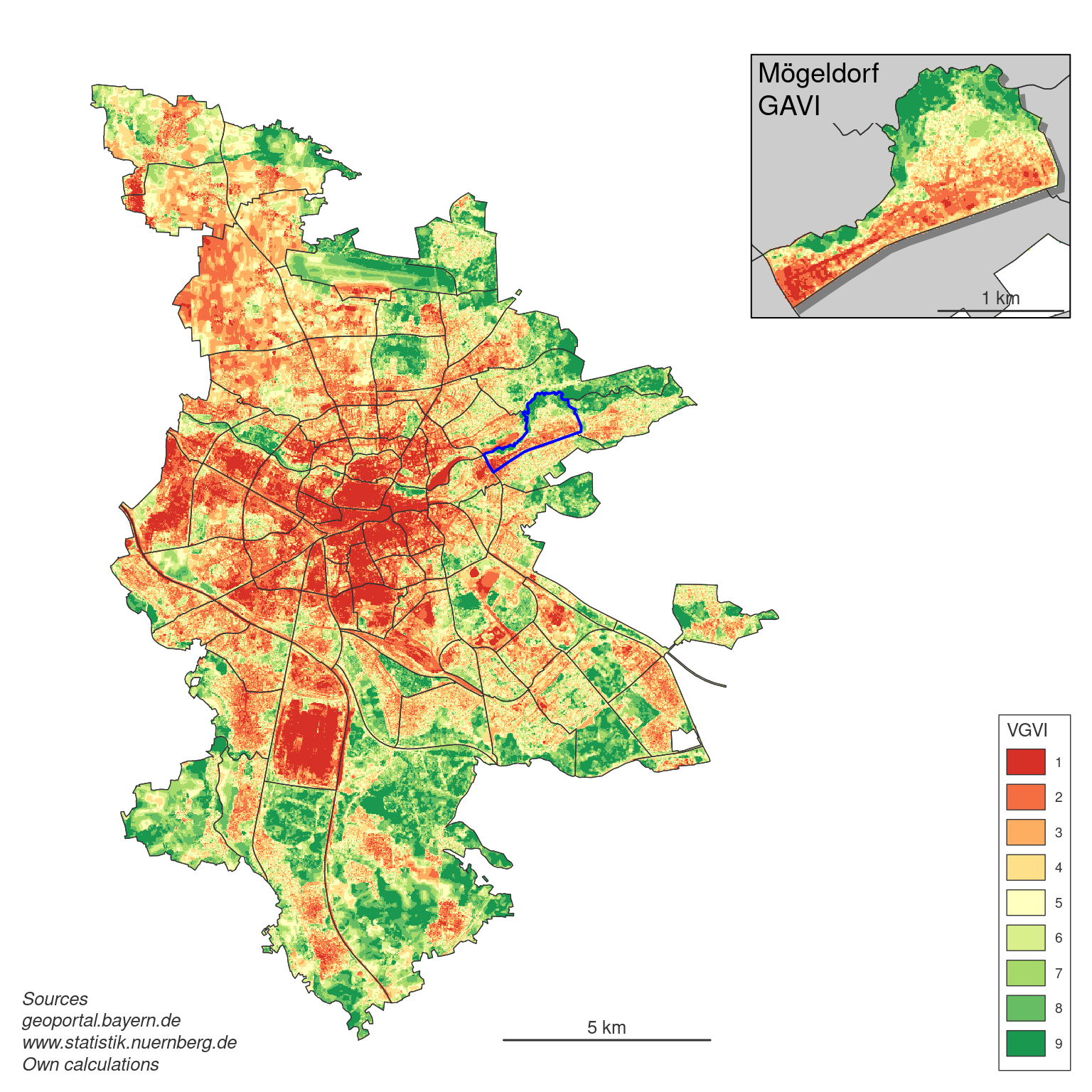
Below is the final VGVI map for Nürnberg, showing how much greenspace is visible from an eye-level perspective at each location. Areas in red represent lower greenness visibility, whereas green areas indicate higher greenness visibility. As expected, more densely built-up districts near the city center display lower VGVI values, while peripheral areas - which often have less building coverage and more open space - reveal higher VGVI values.

Overall, this view-dependent approach highlights not only where greenspace is located, but also how much of it is actually visible to an individual walking through the city - critical information for urban design, mental health research, and ecological planning.

References

Brinkmann, Sebastian T., Dominik Kremer, and Blake Byron Walker. 2022. “Modelling Eye-Level Visibility of Urban Green Space: Optimising City-Wide Point-Based Viewshed Computations Through Prototyping.” AGILE: GIScience Series 3 (June): 1–7. https://doi.org/10.5194/agile-giss-3-27-2022.
Cimburova, Zofie, and Stefan Blumentrath. 2022. “Viewshed-Based Modelling of Visual Exposure to Urban Greenery An Efficient GIS Tool for Practical Planning Applications.” Landscape and Urban Planning 222 (June): 104395. https://doi.org/10.1016/j.landurbplan.2022.104395.
Dadvand, Payam, Xavier Bartoll, Xavier Basagaña, Albert Dalmau-Bueno, David Martinez, Albert Ambros, Marta Cirach, et al. 2016. “Green Spaces and General Health: Roles of Mental Health Status, Social Support, and Physical Activity.” Environment International 91 (May): 161–67. https://doi.org/10.1016/j.envint.2016.02.029.
Hartmann, K., J. Krois, and B. Waske. 2018. “E-Learning Project SOGA: Statistics and Geospatial Data Analysis.” Department of Geographiy, University of Kansas Occasional Paper. https://www.geo.fu-berlin.de/en/v/soga/Geodata-analysis/geostatistics/index.html.
Kaplan, R., and S. Kaplan. 1989. “The Experience of Nature: A Psychological Perspective.” New York: Cambridge University Press.
Labib, S. M., Jonny J. Huck, and Sarah Lindley. 2021. “Modelling and Mapping Eye-Level Greenness Visibility Exposure Using Multi-Source Data at High Spatial Resolutions.” Science of The Total Environment 755 (February): 143050. https://doi.org/10.1016/j.scitotenv.2020.143050.
Li, Xiaojiang, Chuanrong Zhang, Weidong Li, Robert Ricard, Qingyan Meng, and Weixing Zhang. 2015. “Assessing Street-Level Urban Greenery Using Google Street View and a Modified Green View Index.” Urban Forestry & Urban Greening 14 (3): 675–85. https://doi.org/10.1016/j.ufug.2015.06.006.
Markevych, Iana, Julia Schoierer, Terry Hartig, Alexandra Chudnovsky, Perry Hystad, Angel M. Dzhambov, Sjerp de Vries, et al. 2017. “Exploring Pathways Linking Greenspace to Health: Theoretical and Methodological Guidance.” Environmental Research 158 (October): 301–17. https://doi.org/10.1016/j.envres.2017.06.028.
Tabrizian, Payam, Perver K. Baran, Derek Van Berkel, Helena Mitasova, and Ross Meentemeyer. 2020. “Modeling Restorative Potential of Urban Environments by Coupling Viewscape Analysis of Lidar Data with Experiments in Immersive Virtual Environments.” Landscape and Urban Planning 195 (March): 103704. https://doi.org/10.1016/j.landurbplan.2019.103704.
Ulrich, Roger S. 1981. “Natural Versus Urban Scenes.” Environment and Behavior 13 (5): 523–56. https://doi.org/10.1177/0013916581135001.
Ulrich, Roger S., Robert F. Simons, Barbara D. Losito, Evelyn Fiorito, Mark A. Miles, and Michael Zelson. 1991. “Stress Recovery During Exposure to Natural and Urban Environments.” Journal of Environmental Psychology 11 (3): 201–30. https://doi.org/10.1016/s0272-4944(05)80184-7.