Nürnberg - 3. Greenness Accessibility Index (GACI)

library(sf)
library(dplyr)
library(terra)
library(CGEI)

data_repo <- "https://github.com/STBrinkmann/SpatData_Nbg/raw/refs/heads/master/01_analysis/0102_data/02_processed/"

# AOI
aoi <- read_sf(paste0(data_repo, "01_Nbg_Bezirke.gpkg")) %>%
  filter(code_bez != "97") %>% # This is not available in the GAVI
  group_by(code_bez, name_bez) %>%
  summarise() %>%
  ungroup()

# Water mask
water_mask <- read_sf(paste0(data_repo, "02_Nbg_Water.gpkg"))

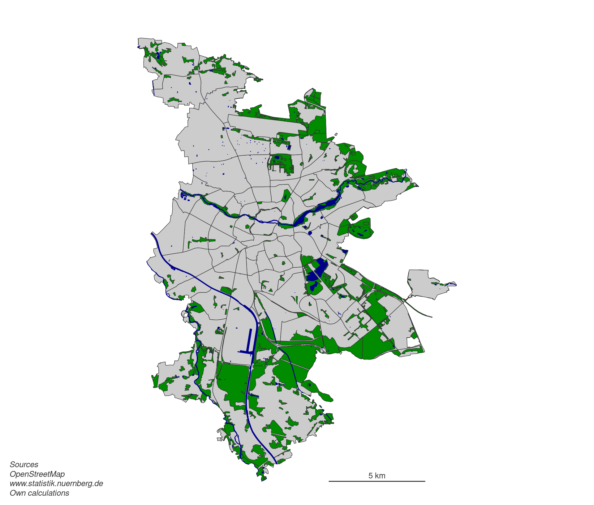
# Parks (>1ha)
osm_parks <- read_sf(paste0(data_repo, "02_Nbg_Greenspace.gpkg")) %>%
  mutate(name = stringr::str_pad(1:n(), 3, pad = "0")) %>%
  mutate(size_ha = st_area(geom) %>%
           units::set_units(value = ha) %>%
           as.numeric()) %>%
  filter(size_ha > 1) %>%
  mutate(size_log = log(size_ha)) %>%
  relocate(geom, .after = last_col())

# --- 1. Generate Road Network & Park Access Points ---

# A. Create buffered AOI boundary to mitigate edge effects
aoi_bbox <- aoi %>%
  st_buffer(5000) %>%
  st_transform(4326) %>%
  st_bbox()

# B. Download and filter OSM road network for walkable paths
osm_roads_raw <- opq(bbox = aoi_bbox) %>%
  add_osm_feature(key = "highway") %>%
  osmdata_sf(quiet = FALSE) %>%
  osm_poly2line()

osm_roads <- osm_roads_raw$osm_lines %>%
  select(highway) %>%
  filter(!highway %in% c("motorway", "motorway_link", "trunk", "trunk_link", "raceway")) %>%
  st_transform(st_crs(aoi)) %>%
  st_intersection(st_buffer(aoi, 5000))

# C. Segment roads for higher intersection accuracy
cores <- 12
if (Sys.info()[["sysname"]] == "Windows") {
  cl <- parallel::makeCluster(cores)
  osm_roads <- suppressWarnings(split(osm_roads, seq(from = 1, to = nrow(osm_roads), by = 200)))
  osm_roads <- parallel::parLapply(cl, osm_roads, function(x){
    nngeo::st_segments(sf::st_cast(x, "LINESTRING"), progress = FALSE)
  })
  parallel::stopCluster(cl)
} else {
  osm_roads <- suppressWarnings(split(osm_roads, seq(from = 1, to = nrow(osm_roads), by = 200))) %>%
    parallel::mclapply(function(x){
      nngeo::st_segments(sf::st_cast(x, "LINESTRING"), progress = FALSE)
    },
    mc.cores = cores, mc.preschedule = TRUE)
}

osm_roads <- st_as_sf(dplyr::as_tibble(data.table::rbindlist(osm_roads)))
osm_roads <- st_set_geometry(osm_roads, "geom")

st_geometry(osm_roads) <- st_geometry(osm_roads) %>%
  lapply(function(x) round(x, 0)) %>%
  st_sfc(crs = st_crs(osm_roads))

# D. Derive park centroids and road intersections
osm_park_centroids <- osm_parks %>%
  st_centroid() %>%
  select(name, size_ha, size_log)

# Helper function
st_multipoint_to_point <- function(x) {
  x.points <- x[which(sf::st_geometry_type(x) == "POINT"), ]
  x.multipoints <- x[which(sf::st_geometry_type(x) == "MULTIPOINT"), ]

  for (i in 1:nrow(x.multipoints)) {
    x.points <- x.points %>%
      dplyr::add_row(sf::st_cast(x.multipoints[i, ], "POINT"))
  }

  return(x.points)
}

osm_park_road_interesect <- osm_parks %>%
  st_boundary() %>%
  st_intersection(osm_roads) %>%
  select(name, size_ha, size_log) %>%
  st_multipoint_to_point()

# E. Combine both into final access point layer
park_accesspoints <- rbind(osm_park_centroids, osm_park_road_interesect)

# --- 2. Prepare Observer Locations ---

# A. Create a regular grid (10m resolution)
observer <- st_make_grid(aoi, cellsize = 50, what = "centers") %>%
  st_as_sf() %>%
  st_set_geometry("geom")
observer <- observer[aoi,]
observer <- observer %>%
  mutate(id = 1:n()) %>%
  relocate(id, .after = last_col())

# B. Remove points inside parks
obs_in_parks <- observer[osm_parks, ]
observer <- observer[-obs_in_parks$id, ]

# C. Remove points in water bodies
observer <- observer[-(observer[water_mask, ]$id), ]

# Download OSM data for your region of interest
if(!file.exists("01_analysis/0101_data/osrm/mittelfranken-latest.osm.pbf")){
  dir.create("01_analysis/0101_data/osrm/", showWarnings = FALSE)
  default_timeout <- getOption("timeout")
  options(timeout = max(600, default_timeout))
  download.file(
    url = "https://download.geofabrik.de/europe/germany/bayern/mittelfranken-latest.osm.pbf",
    destfile = "01_analysis/0101_data/osrm/mittelfranken-latest.osm.pbf",
    mode="wb"
  )
  options(timeout = default_timeout)
}

# OSRM Docker commands:
# 1) Navigate to the appropriate folder:
#    cd 01_analysis/0101_data/osrm/
# 2) Extract, partition, and customize:
#    sudo docker run -t -v "${PWD}:/data" osrm/osrm-backend osrm-extract -p /opt/foot.lua /data/mittelfranken-latest.osm.pbf
#    sudo docker run -t -v "${PWD}:/data" osrm/osrm-backend osrm-partition /data/mittelfranken-latest.osrm
#    sudo docker run -t -v "${PWD}:/data" osrm/osrm-backend osrm-customize /data/mittelfranken-latest.osrm
# 3) Run the OSRM server:
#    sudo docker run -t -i -p 5000:5000 -v "${PWD}:/data" osrm/osrm-backend osrm-routed --max-table-size=50000 --algorithm mld /data/mittelfranken-latest.osrm

# --- 3. Network Analysis with OSRM ---

# The OSRM server is run locally via Docker (setup described earlier).

observer_park_duration <- function(j){
  # Identify k-nearest access points
  knn_access <- nngeo::st_nn(
    observer[j,],
    park_accesspoints,
    k = 2 * round(sqrt(nrow(park_accesspoints))),
    progress = FALSE
  ) %>% unlist()

  # Compute travel times using OSRM
  duration_table <- osrmTable(
    src = observer[j,],
    dst = park_accesspoints[knn_access,],
    osrm.server = "http://0.0.0.0:5000/",
    osrm.profile = "foot"
  )

  # Select best match (close & large)
  out <- tibble(
    id = observer[j,]$id,
    dist = as.numeric(duration_table$durations),
    size_ha = park_accesspoints[knn_access,]$size_ha,
    size_log = park_accesspoints[knn_access,]$size_log,
    name = park_accesspoints[knn_access,]$name
  ) %>%
    group_by(name) %>%
    filter(dist == min(dist)) %>%
    distinct() %>%
    ungroup() %>%
    # Normalize distance & size values
    mutate(dist_01 = dist / mean(dist) * 100,
           size_01 = size_log / mean(size_log) * 100) %>%
    mutate(dist_01 = 1 - dist_01 / max(dist_01),
           size_01 = size_01 / max(size_01)) %>%
    # Weight by distance vs. park size
    mutate(w = (1.91 / 0.85 * dist_01 + size_01) / 2) %>%
    filter(w == max(w)) %>%
    select(id, name, dist, size_ha, w)

  return(out)
}

# Split observer set into manageable chunks
obs_seq <- split(1:nrow(observer), ceiling(seq_along(1:nrow(observer))/250))

# Initialize an output CSV
tibble(
  id = as.numeric(),
  name = as.character(),
  dist = as.numeric(),
  size_ha = as.numeric(),
  w = as.numeric()
) %>%
  readr::write_csv("01_analysis/0101_data/osrm/access_table.csv", col_names = TRUE)

# Parallel loop over observer subsets
pb = pbmcapply::progressBar(min = 0, max = length(obs_seq))
stepi = 1
for(this_seq in obs_seq){
  dist_table <- parallel::mclapply(this_seq, observer_park_duration, mc.cores = 18) %>%
    do.call(rbind, .)

  readr::write_csv(dist_table, "01_analysis/0101_data/osrm/access_table.csv", append = TRUE)
  setTxtProgressBar(pb, stepi)
  stepi = stepi + 1
}
close(pb)

# Merge distance results with the observer SF
dist_table <- readr::read_csv("01_analysis/0101_data/osrm/access_table.csv")
dist_sf <- inner_join(observer, dist_table)

# Terminate OSRM server and cleanup if desired
unlink("01_analysis/0101_data/osrm/", recursive = TRUE)

# --- 4. Convert Access Values to GACI Raster ---

# A. Interpolate to 10m grid using IDW
gaci_raw <- CGEI::sf_interpolat_IDW(
  observer = dist_sf,
  v = "w",
  aoi = aoi,
  max_distance = Inf,
  n = 20,
  raster_res = 10,
  na_only = TRUE,
  cores = 22,
  progress = TRUE
)

# B. Park cells: assign ideal accessibility
park_cells <- terra::extract(gaci_raw, osm_parks, cells = TRUE, ID = FALSE)$cell
gaci_raw[park_cells] <- NA

# C. Reclassify via Jenks for readability
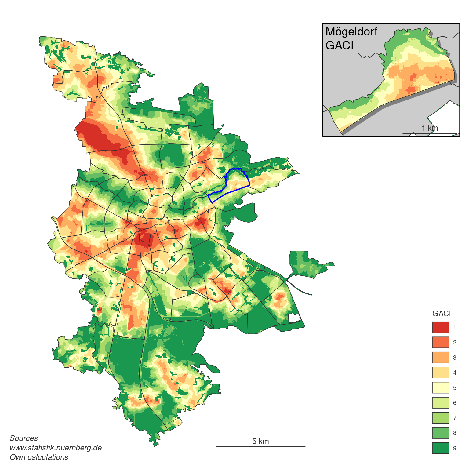
gaci <- CGEI:::reclassify_jenks(gaci_raw, n_classes = 9)
gaci[park_cells] <- 9

gaci <- gaci %>%
  crop(aoi) %>%
  mask(aoi)
names(gaci) <- "GACI"

References

Duncan, Michael, Neil Clarke, Samantha Birch, Jason Tallis, Joanne Hankey, Elizabeth Bryant, and Emma Eyre. 2014. “The Effect of Green Exercise on Blood Pressure, Heart Rate and Mood State in Primary School Children.” International Journal of Environmental Research and Public Health 11 (4): 3678–88. https://doi.org/10.3390/ijerph110403678.
Fone, D., J. White, D. Farewell, M. Kelly, G. John, K. Lloyd, G. Williams, and F. Dunstan. 2014. “Effect of Neighbourhood Deprivation and Social Cohesion on Mental Health Inequality: A Multilevel Population-Based Longitudinal Study.” Psychological Medicine 44 (11): 2449–60. https://doi.org/10.1017/s0033291713003255.
Giles-Corti, Billie, Melissa H. Broomhall, Matthew Knuiman, Catherine Collins, Kate Douglas, Kevin Ng, Andrea Lange, and Robert J. Donovan. 2005. “Increasing Walking.” American Journal of Preventive Medicine 28 (2): 169–76. https://doi.org/10.1016/j.amepre.2004.10.018.
Holtan, Meghan T., Susan L. Dieterlen, and William C. Sullivan. 2014. “Social Life Under Cover.” Environment and Behavior 47 (5): 502–25. https://doi.org/10.1177/0013916513518064.
Kingsbury, Mila, Zahra Clayborne, Ian Colman, and James B. Kirkbride. 2019. “The Protective Effect of Neighbourhood Social Cohesion on Adolescent Mental Health Following Stressful Life Events.” Psychological Medicine 50 (8): 1292–99. https://doi.org/10.1017/s0033291719001235.
Labib, S. M., Sarah Lindley, and Jonny J. Huck. 2020. “Spatial Dimensions of the Influence of Urban Green-Blue Spaces on Human Health: A Systematic Review.” Environmental Research 180 (January): 108869. https://doi.org/10.1016/j.envres.2019.108869.
———. 2021. “Estimating Multiple Greenspace Exposure Types and Their Associations with Neighbourhood Premature Mortality: A Socioecological Study.” Science of The Total Environment 789 (October): 147919. https://doi.org/10.1016/j.scitotenv.2021.147919.
Lachowycz, K., and A. P. Jones. 2011. “Greenspace and Obesity: A Systematic Review of the Evidence.” Obesity Reviews 12 (5): e183–89. https://doi.org/10.1111/j.1467-789x.2010.00827.x.
Markevych, Iana, Julia Schoierer, Terry Hartig, Alexandra Chudnovsky, Perry Hystad, Angel M. Dzhambov, Sjerp de Vries, et al. 2017. “Exploring Pathways Linking Greenspace to Health: Theoretical and Methodological Guidance.” Environmental Research 158 (October): 301–17. https://doi.org/10.1016/j.envres.2017.06.028.
McGrath, Leslie J., Will G. Hopkins, and Erica A. Hinckson. 2015. “Associations of Objectively Measured Built-Environment Attributes with Youth ModerateVigorous Physical Activity: A Systematic Review and Meta-Analysis.” Sports Medicine 45 (6): 841–65. https://doi.org/10.1007/s40279-015-0301-3.
Mitchell, Richard. 2013. “Is Physical Activity in Natural Environments Better for Mental Health Than Physical Activity in Other Environments?” Social Science & Medicine 91 (August): 130–34. https://doi.org/10.1016/j.socscimed.2012.04.012.
Pretty, Jules, Jo Peacock, Martin Sellens, and Murray Griffin. 2005. “The Mental and Physical Health Outcomes of Green Exercise.” International Journal of Environmental Health Research 15 (5): 319–37. https://doi.org/10.1080/09603120500155963.
Weinstein, Netta, Andrew Balmford, Cody R. DeHaan, Valerie Gladwell, Richard B. Bradbury, and Tatsuya Amano. 2015. “Seeing Community for the Trees: The Links Among Contact with Natural Environments, Community Cohesion, and Crime.” BioScience 65 (12): 1141–53. https://doi.org/10.1093/biosci/biv151.
Williams, Andrew James, Kath Maguire, Karyn Morrissey, Tim Taylor, and Katrina Wyatt. 2020. “Social Cohesion, Mental Wellbeing and Health-Related Quality of Life Among a Cohort of Social Housing Residents in Cornwall: A Cross Sectional Study.” BMC Public Health 20 (1). https://doi.org/10.1186/s12889-020-09078-6.