Visibility - Sensitivity Analysis
Introduction
Visibility analyses are powerful tools in spatial research that help us understand what can be seen from a particular point in the landscape. For my Bachelor Thesis, I am investigating how visible green- and bluespaces influence mental health, using data from a medical study in Vancouver. The study area includes Vancouver City, Burnaby, and Surrey. Specifically, I use the Viewshed Greenness Visibility Index (VGVI) to capture the proportion of visible greenness within a particular viewshed.
However, an important challenge arises when scaling visibility analyses to cover large areas or many points: computational cost. High-resolution rasters and large viewing distances dramatically increase the number of cells to check, resulting in lengthy processing times. In such scenarios, running a sensitivity analysis is beneficial to understand how certain parameters — especially maximum distance and raster resolution — affect both accuracy and computational load. By doing this, we can:
- Identify parameter values that keep computation times within practical limits.
- Capture visibility in a way that is meaningful for understanding the local geography (e.g., typical line-of-sight distances in the urban environment of your study area).
Below, I explain how to systematically evaluate the influence of different distances and resolutions on viewshed calculations and why this step is critical for large-scale studies like the one I am conducting in Vancouver.

To analyze the effect of visible greenness, I’ll be using the VGVI. This index expresses the proportion of visible greenness to the total visible area based on a viewshed. VGVI values range from 0 to 1, with 0 indicating that no green cells are visible and 1 meaning all visible cells are green. A detailed example of how to calculate the VGVI can be found in a recent post and in my CGEI R package.
Because VGVI relies on a viewshed, the analysis requires a Digital Surface Model (DSM), a Digital Terrain Model (DTM), and the observer location. Conceptually, the viewshed function checks every point within a defined radius (the maximum distance) to determine if it is visible from the observer’s vantage point.
# Load libraries
library(dplyr)
library(ggplot2)
library(sf)
library(CGEI)
library(terra)

# Load DSM and DEM
dsm <- rast("/mnt/p/R/Remote Sensing Data/Vancouver/DSM_Vancouver_1m.tif")
dtm <- rast("/mnt/p/R/Remote Sensing Data/Vancouver/DTM_Vancouver_1m.tif")

# Sample observer location
st_observer <- sfheaders::sf_point(c(487616.2, 5455970)) %>%
    st_sf(crs = st_crs(26910))

# Compute Viewshed
viewshed_1 <- CGEI::viewshed_list(observer = st_observer,
                                  dsm_rast = dsm, dtm_rast = dtm,
                                  max_distance = 250, observer_height = 1.7)
plot(viewshed_1[[1]])
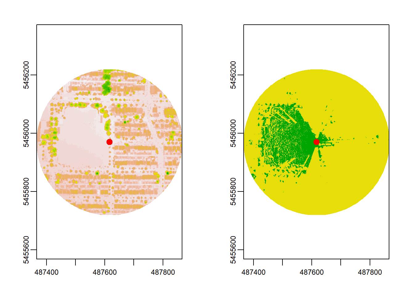
Above, the left plot shows the DSM for a local area, and the right plot highlights visibility in green (visible) and yellow (not visible). The observer (marked as a red dot) has an extensive view toward the west but limited visibility to the east.
Next, the VGVI calculation typically follows by overlaying a greenspace mask on the viewshed. This post, however, focuses on understanding two crucial parameters for viewshed calculations: distance (the radius around each point to be considered) and resolution (the level of spatial detail in the raster data).
Sensitivity Analysis
A few points can be handled quickly at high resolution and large distance (e.g., 800 m at 1 m resolution might take just a few seconds). But when dealing with an entire city — like Vancouver — the same approach can lead to massive computation times. Below is a systematic exploration of how distance and resolution impact visibility analysis.
Samples
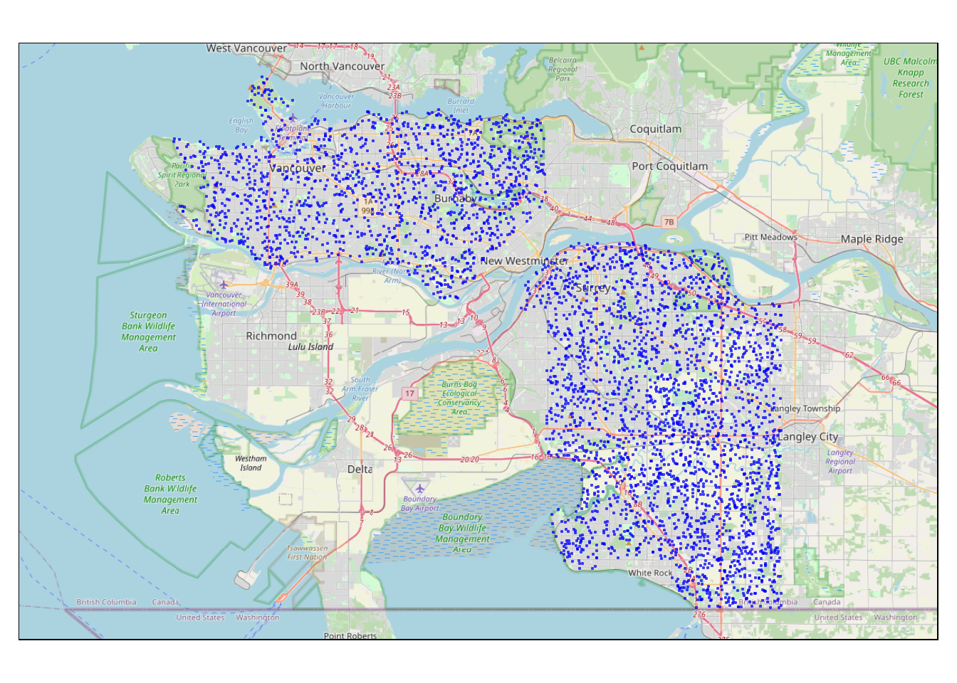
To illustrate the sensitivity analysis, I drew a representative sample of 4000 observer locations across the study area:
sf_sample <- st_make_grid(aoi, 250, what = "centers")

sf_sample <- sf_sample[aoi,] %>%
  st_as_sf() %>%
  st_intersection(aoi)

set.seed(1234)
sf_sample <- sf_sample %>%
  group_by(region) %>%
  sample_n(2000) %>%
  ungroup()
##
## ── tmap v3 code detected ───────────────────────────────────────────────────────
## [v3->v4] `tm_dots()`: use `fill_alpha` instead of `alpha`.
Distance
In a previous example, a 250 m distance was used. What happens if we increase the maximum distance to 800 m?
# Compute Viewshed
viewshed_2 <- CGEI::viewshed_list(observer = st_observer,
                                  dsm_rast = dsm, dtm_rast = dtm,
                                  max_distance = 800, observer_height = 1.7)
plot(viewshed_2[[1]])
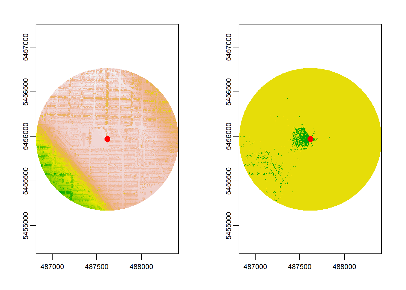
Here, increasing the distance to 800 m doesn’t reveal much more visible area for this particular observer location compared to 250 m. In other words, beyond 250 m, there isn’t significant new visibility to be gained. But the computation time dropped from around ~1200 ms to ~80 ms!
This illustrates that maximum distance is not just a random choice—it must be guided by the real-world context. For instance, if you expect most relevant visibility influences (e.g., green spaces) to be within a few hundred meters, using very large radii might not add detail but will consume a lot more compute resources. In urban planning and health studies, visibility beyond a certain threshold can be less relevant because the eye-level environment that truly impacts people often lies closer.
Below is a function to quantify the proportion of visible area for each distance value in the viewshed:
visibleDistance <- function(x) {
  # Get XY coordinates of cells
  xy <- terra::xyFromCell(x, which(!is.na(x[])))

  # Calculate euclidean distance from observer to cells
  centroid <- colMeans(terra::xyFromCell(x, which(!is.na(x[]))))
  dxy = round(sqrt((centroid[1] - xy[,1])^2 + (centroid[2] - xy[,2])^2))
  dxy[dxy==0] = min(dxy[dxy!=0])

  # Combine distance and value
  cbind(dxy, unlist(terra::extract(x, xy), use.names = FALSE)) %>%
    as_tibble() %>%
    rename(visible = V2) %>%
    arrange(dxy) %>%
    group_by(dxy) %>%
    # Mean visible area for each distinct distance value
    summarise(visible = mean(visible)) %>%
    ungroup() %>%
    return()
}
We can apply it to the 800 m viewshed:
| Distance | Visibility |
|---|---|
| 1 | 100.0% |
| 2 | 100.0% |
| 3 | 100.0% |
| 4 | 100.0% |
| 5 | 100.0% |
| 795 | 0.2% |
| 796 | 0.2% |
| 797 | 0.0% |
| 798 | 0.1% |
| 799 | 0.1% |
Next, I extend this logic across all 4000 sample points, computing the viewshed and proportion of visible area for each distance value. This chunk runs the analysis in smaller “chunks” to work around RAM limitations:
chunks <- st_make_grid(aoi, 5000, what = "polygons")
chunks <- chunks[aoi,]
out <- tibble(
  dxy = numeric(),
  visible = numeric()
)

for(i in seq_along(chunks)) {
  cat("\r", stringr::str_pad(i, 2), "|", length(chunks))

  if(nrow(sf_sample[chunks[i],]) == 0) next
  # Viewshed
  this_vs <- CGEI::viewshed_list(observer = sf_sample[chunks[i],],
                                 dsm_rast = dsm, dtm_rast = dtm,
                                 max_distance = 800, observer_height = 1.7,
                                 cores = 22)

  # Visible area
  this_dist <- lapply(this_vs, visibleDistance) %>%
    do.call(rbind, .)

  # Add to "out"
  out <- rbind(out, this_dist)
}
The following plot shows how visibility generally decreases with increasing distance. Notably, there are local “bumps” at around 250 m and 500 m, possibly due to Vancouver’s urban planning and distribution of parks.
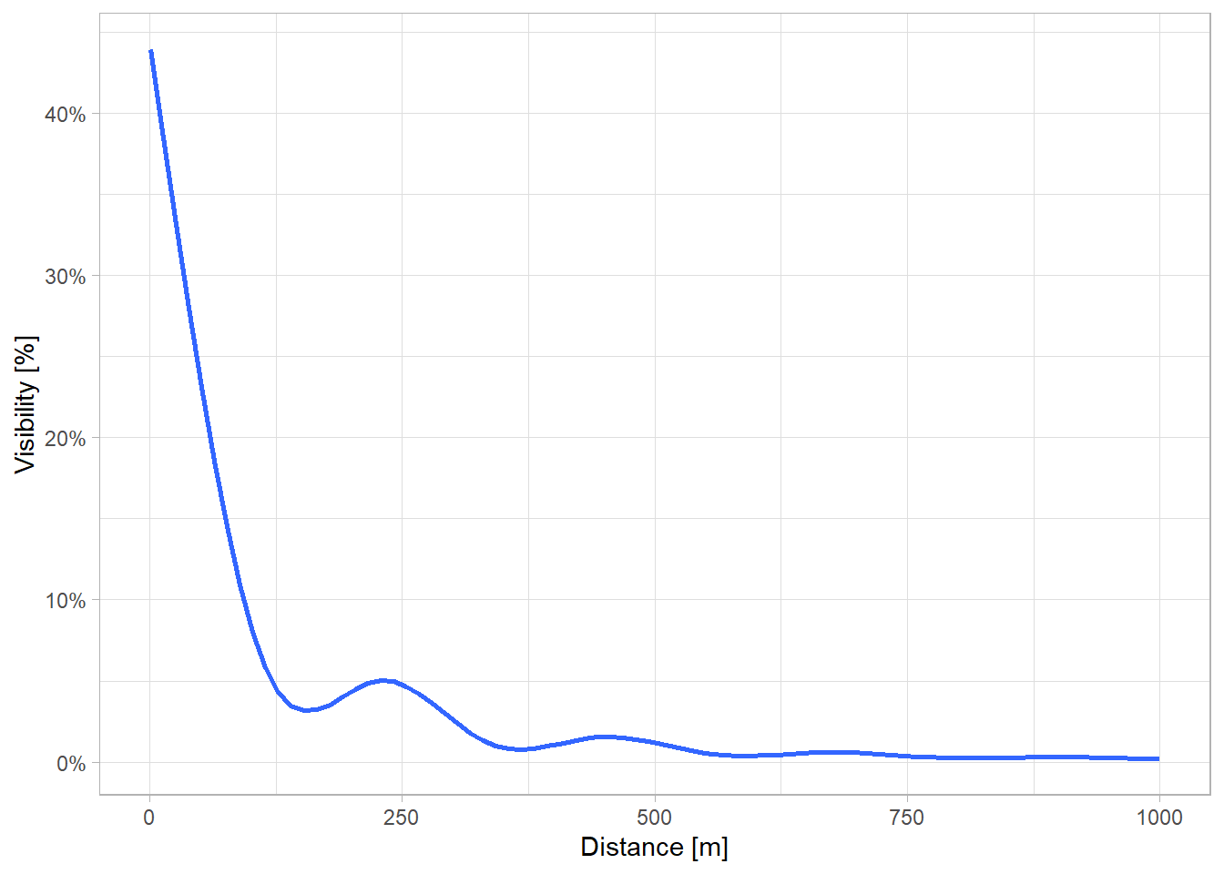
Given these findings, I have chosen a distance threshold of 550 meters — a point that appears to capture most of the visibility in this study area without incurring the full computational cost of an 800 m radius. In real-world terms, 550 m can be considered a reasonable walking distance within an urban environment, aligning with the idea that this radius covers the bulk of directly perceptible green space around a person.
Resolution
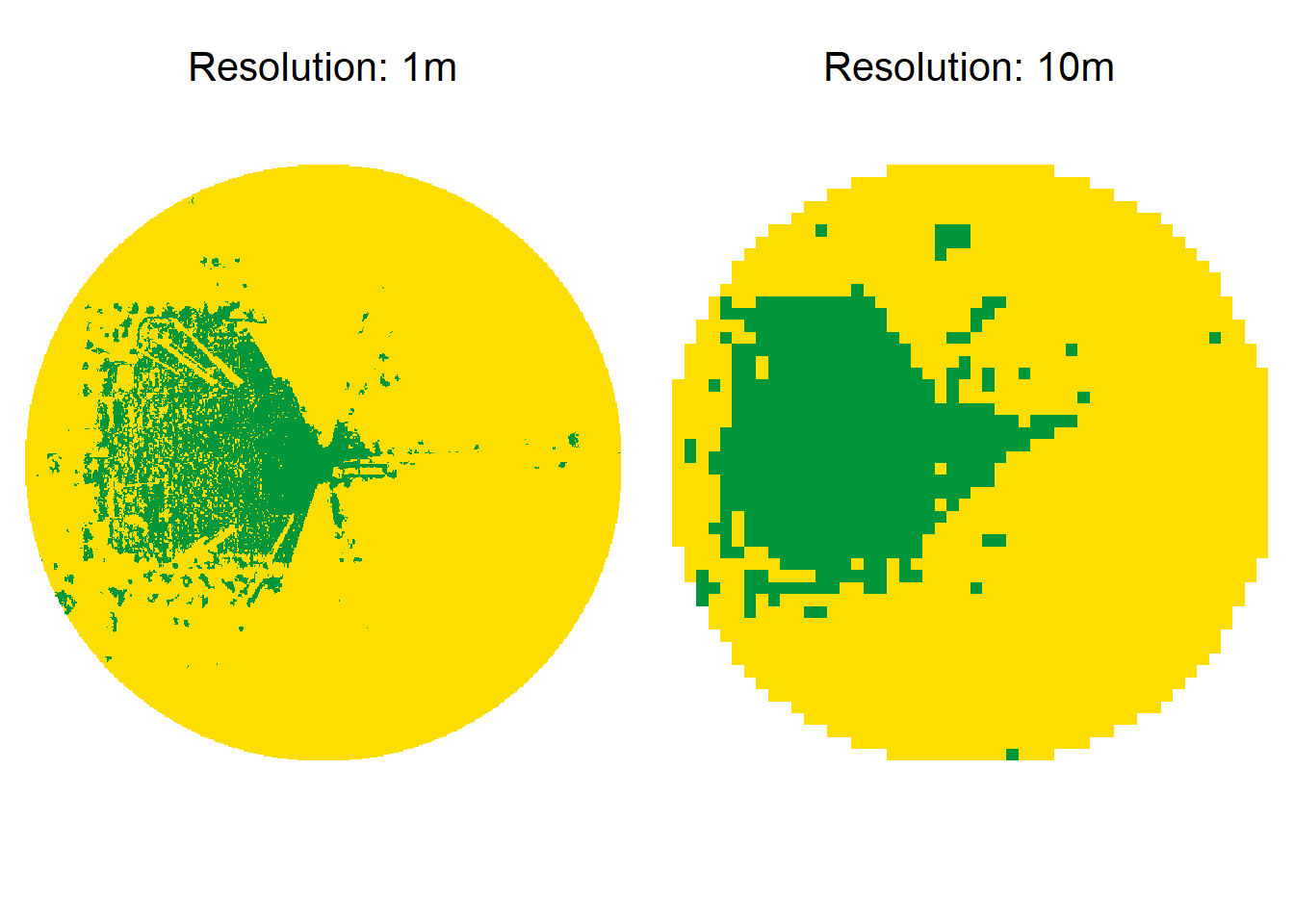
The resolution parameter determines how coarsely or finely the DSM and DTM are aggregated. Higher resolutions (e.g., 1 m) produce more precise visibility maps but also mean more cells to process. Conversely, coarser resolutions (e.g., 10 m) involve significantly fewer cells—thus less computation time—but come at the cost of spatial detail.
For instance, at a 1 m resolution within a 550 m radius, you would have ~1,210,000 cells and might spend 0.5 seconds per viewshed. At 10 m resolution, there are only ~12,100 cells, and it might take just 0.01 seconds to compute. Below is a direct visualization of 1 m vs. 10 m resolution at a 250 m distance radius:
To quantify these differences, I compare visibility grids of various resolutions to the 1 m baseline:
compare_resolution <- function(observer, dsm_path, dtm_path) {
  viewshed_tbl <- lapply(c(1, 2, 5, 10), FUN = function(x) {
    # Load and aggregate DSM and DTM
    tmp_dsm <- dsm_path %>% rast() %>% crop(st_buffer(observer, 550)) %>% aggregate(x)
    tmp_dtm <- dtm_path %>% rast() %>% crop(st_buffer(observer, 550)) %>% aggregate(x)

    # Get values of viewshed with resolution x
    time_a <- Sys.time()
    all_value <- CGEI::viewshed_list(observer = observer,
                                     dsm_rast = tmp_dsm, dtm_rast = tmp_dtm,
                                     max_distance = 550, observer_height = 1.7)
    time_b <- Sys.time()
    all_value <- all_value %>%
      purrr::pluck(1) %>%
      terra::values(na.rm = TRUE)

    # Return Distance, proportion of visible area and computation time
    return(tibble(
      Resolution = x,
      Similarity = length(which(all_value == 1)) / length(all_value),
      Time = as.numeric(difftime(time_b, time_a, units = "secs"))
    ))
  }) %>%
    do.call(rbind, .)

  viewshed_tbl %>%
    rowwise() %>%
    mutate(Similarity = min(viewshed_tbl[1,2], Similarity) / max(viewshed_tbl[1,2], Similarity)) %>%
    return()
}
The boxplots below show that similarity decreases as resolution gets coarser. Meanwhile, computation time greatly benefits from lower resolutions. On average, the mean computation time for 1 m, 2 m, 5 m, and 10 m resolutions is approximately 4.80s, 1.05s, 0.85s, and 0.75s, respectively. A 2 m resolution offers a good balance for this analysis — about ~75% similarity to the baseline but only about 1/5 of the computation time.

Conclusion
Conducting large-scale viewshed analyses — like computing the VGVI for an entire metropolitan region — can quickly become computationally expensive, so optimally choosing distance and resolution is essential. A sensitivity analysis helps pinpoint thresholds that capture the real-world visibility context while managing processing times.
In this study, evaluating Vancouver’s diverse landscapes showed that beyond ~550 m, little additional visibility is gained, so 550 m became the selected maximum distance. For raster resolution, 2 m appeared to balance reasonable similarity to a 1 m baseline with a fivefold decrease in runtime.
These decisions have practical significance. They mean that:
- We are capturing the bulk of relevant visibility without overly large viewshed radii.
- We retain enough spatial detail with a 2 m resolution to reflect real-world conditions without ballooning our computation costs.
Given that my complete study area contains roughly 108 million points, even these “optimized” parameters translate to about 20 days on a high-performance server. Taking the time to conduct a sensitivity analysis before launching into massive computations is therefore invaluable. It ensures that key parameters—like distance and resolution—are set in a scientifically and practically sound manner, minimizing wasted resources and providing results that more accurately reflect real-world visibility patterns.