Nürnberg - 2. Greenspace Availability Index (GAVI)

Introduction

Greenspace availability plays a critical role in understanding the impact of urban environments on human health and well-being. One common approach to measuring greenspace availability is through simple 2D buffer analyses around residential or workplace locations using remote sensing data, such as the Normalized Difference Vegetation Index (NDVI) or land-use/land-cover (LULC) maps (Labib, Lindley, and Huck 2020a). These indices help quantify photosynthetically active vegetation and the proportion of green land cover. Moreover, to address seasonal variations and different qualities of greenspace, researchers recommend using multiple remote sensing products at various scales (Markevych et al. 2017; Labib, Lindley, and Huck 2020b). Beyond its general relevance for urban public health, greenspace availability is especially vital for mitigating environmental stressors - an important aspect of reducing harm in cities (Markevych et al. 2017).

Urban areas are often associated with elevated levels of air pollution, heat, and noise - factors that can negatively impact mental and physical health (Dadvand and Nieuwenhuijsen 2019). Studies indicate that higher concentrations of greenspace help reduce traffic-related air pollution through plant uptake and deposition on leaf surfaces (Givoni 1991; Paoletti et al. 2011; Nowak et al. 2014). Consequently, air pollutant concentrations are generally lower in greener areas, and exposure to greenspace near schools and residential districts can mitigate adverse effects such as depression and cognitive deficits in children (Su et al. 2011; Dadvand et al. 2012, 2015; Ali and Khoja 2019). Furthermore, the urban heat island effect, mainly caused by the replacement of vegetation with built-up infrastructure like concrete and high-rise buildings, exacerbates local temperatures and reduces wind flow (Voogt and Oke 2003; Phelan et al. 2015; Heaviside, Macintyre, and Vardoulakis 2017). Exposure to high temperatures is linked to increased hospital admissions and mortality (Basu 2009; D’Ippoliti et al. 2010), and there is emerging evidence of elevated mental health risks during extreme heat events (Nori-Sarma et al. 2022). Together, these findings underscore the importance of incorporating greenspace into urban planning to mitigate environmental stressors and safeguard public health - key considerations for the development of indices such as the GAVI (Greenspace Availability Index).

Data

The relevant spatial datasets have been uploaded on Zenodo: administrative boundaries (AOI), NDVI and LAI rasters, and a binary land-cover raster for greenspace analysis.

library(sf)
library(dplyr)
library(terra)
library(CGEI)

zenodo_url <- "https://zenodo.org/records/14633167/files/"

# AOI
aoi <- read_sf(paste0(zenodo_url, "01_Nbg_Bezirke.gpkg")) %>%
  filter(code_bez != "97") %>% # This is not available in the GAVI
  group_by(code_bez, name_bez) %>%
  summarise() %>%
  ungroup()

# NDVI
ndvi <- rast(paste0(zenodo_url, "03_ndvi_10m.tif"))

# LAI
lai <- rast(paste0(zenodo_url, "03_lai_10m.tif"))

# Greenspace (binary)
lulc <- rast(paste0(zenodo_url, "03_lulc_10m.tif"))

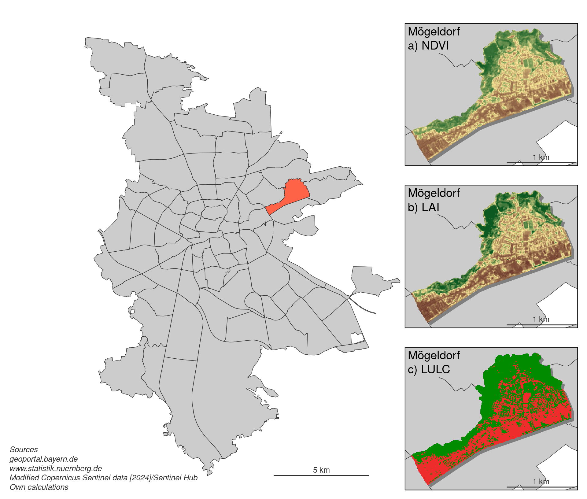
Nürnberg, shown on the left in grey, is divided into 86 administrative districts. Mögeldorf has been highlighted in orange to provide examples of the three key greenness metrics on the right:

1. NDVI highlights areas of more intense photosynthetic activity in greener hues

2. LAI shows the density of foliage based on leaf area

3. LULC distinguishes vegetated areas (green) from non-vegetated surfaces (red)

Lacunarity

Lacunarity is a key measure of spatial heterogeneity - often described as the “gappiness” of a pattern - making it especially useful for characterizing how vegetation is distributed across landscapes (Labib, Lindley, and Huck 2020b; Hoechstetter, Walz, and Thinh 2011). While other measures simply aggregate the amount of greenspace, lacunarity captures differences in the structure of that greenspace. For instance, a continuous patch of trees will exhibit lower lacunarity than an area of fragmented green spots, even if both have the same total leaf cover.

This insight is critically important in urban contexts, where the spatial arrangement of vegetation affects microclimate regulation, air pollution buffering, and recreational opportunities. Moreover, lacunarity helps address the modifiable areal unit problem (MAUP) by examining multiple scales simultaneously. Smaller scales might capture local vegetation buffers (e.g., shrubs along roadways), while larger scales reflect broader landscape connectivity and potential for recreational use.

In practice, lacunarity is calculated by sliding a square window of varying buffer sizes across a raster (e.g., NDVI, LAI, or LULC), then quantifying how homogeneous or heterogeneous each neighborhood is at each scale. The result is a scale-dependent measure of pattern variation. Below is an example of how lacunarity can be computed at five buffer distances (50, 100, 200, 300, and 400 meters) using the CGEI R package:

# Combine rasters
rast_vec <- c(ndvi, lai, lulc)

# Calculate Lacunarity at 5 relevant levels: 50m, 100m, 200m, 300m, 400m
lac_nbg <- lacunarity(rast_vec,
                      r_vec = c(50, 100, 200, 300, 400)/10 * 2 + 1,
                      cores = 22L)

Below is a log–log plot of lacunarity \(𝛬(r)\) against the neighborhood size \(r\). Conceptually, as we increase the size of the moving window (similar to a focal analysis), we average over a larger area, making the image appear more homogeneous - in other words, small-scale patchiness becomes less visible at bigger scales.

From the plot, we see that NDVI and LAI start with relatively high lacunarity and then quickly decline, suggesting that vegetation density becomes more uniform as we “zoom out.” Meanwhile, LULC begins at a higher lacunarity level and still remains above 0.25 at larger distances, meaning binary greenspace (presence or absence) is initially more “patchy” at small scales and smooths out at very larg scales. Overall, all three measures - NDVI, LAI, and LULC - show a reduction in spatial heterogeneity with increasing window size, consistent with the smoothing effect of larger-scale aggregation.

When we combine multiple metrics (e.g., NDVI, LAI, LULC) across multiple scales (e.g., 50 m to 400 m) using lacunarity-based weights, we capture:

1. Different ecosystem functions at different neighborhood sizes - smaller buffers highlight local vegetation that filters pollution and noise, while larger buffers capture larger green spaces like parks.
2. Spatial structure - fragmented or “gappy” greenspace has higher lacunarity at small scales, but becomes more uniform at larger scales.

By assigning individual weights for each metric and scale (based on how patchy they are), we ensure that not all neighborhood sizes contribute equally to people’s overall exposure. This strategy also helps mitigate the Modifiable Areal Unit Problem (MAUP), producing a Greenspace Availability Index (GAVI) that reflects both the quantity of greenspace and its arrangement at scales meaningful for human well-being.

GAVI

# Calculate GAVI
gavi_nbg <- gavi(x = rast_vec, lac_nbg, cores = 22)
names(gavi_nbg) <- "GAVI"

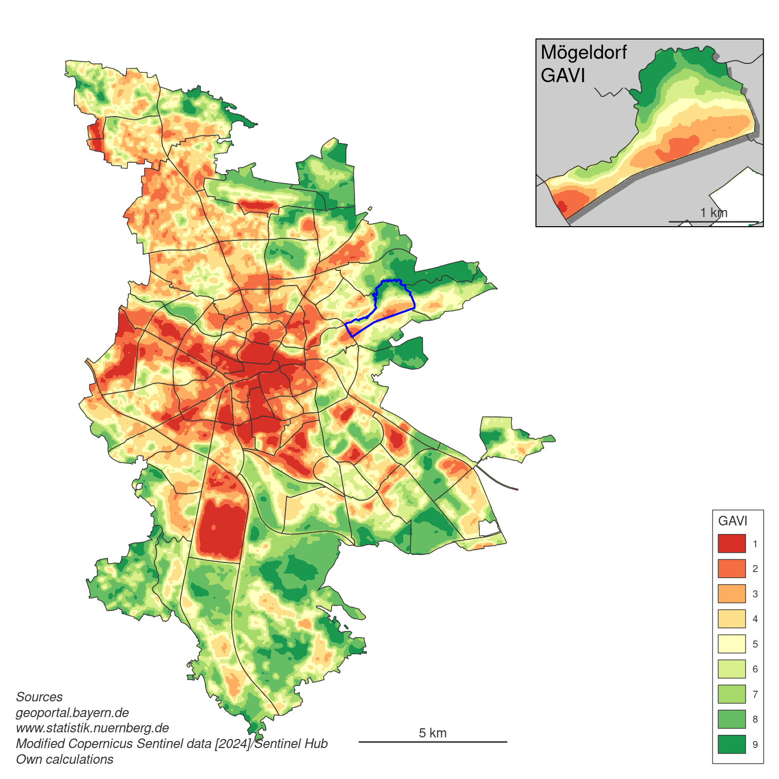
Below is the final Greenspace Availability Index (GAVI) map for Nürnberg, derived by combining NDVI, LAI, and LULC across five spatial scales (50 m to 400 m) using lacunarity-based weights. The map highlights where greenspace is low (red shades, corresponding to lower GAVI values) and high (green shades, corresponding to higher GAVI values). Unsurprisingly, dense urban areas toward the city center show lower greenspace availability, while more peripheral or park-rich districts exhibit higher levels of greenery.

By capturing both the amount and the spatial arrangement of vegetation at multiple neighborhood scales, this multi-scale, multi-metric approach provides a more nuanced picture of greenspace availability - valuable for urban planning, public health, and environmental management.

References

Ali, Naureen A., and Adeel Khoja. 2019. “Growing Evidence for the Impact of Air Pollution on Depression.” Ochsner Journal 19 (1): 4–4. https://doi.org/10.31486/toj.19.0011.
Basu, Rupa. 2009. “High Ambient Temperature and Mortality: A Review of Epidemiologic Studies from 2001 to 2008.” Environmental Health 8 (1). https://doi.org/10.1186/1476-069x-8-40.
D’Ippoliti, Daniela, Paola Michelozzi, Claudia Marino, Francesca de’Donato, Bettina Menne, Klea Katsouyanni, Ursula Kirchmayer, et al. 2010. “The Impact of Heat Waves on Mortality in 9 European Cities: Results from the EuroHEAT Project.” Environmental Health 9 (1). https://doi.org/10.1186/1476-069x-9-37.
Dadvand, Payam, Audrey de Nazelle, Margarita Triguero-Mas, Anna Schembari, Marta Cirach, Elmira Amoly, Francesc Figueras, Xavier Basagaña, Bart Ostro, and Mark Nieuwenhuijsen. 2012. “Surrounding Greenness and Exposure to Air Pollution During Pregnancy: An Analysis of Personal Monitoring Data.” Environmental Health Perspectives 120 (9): 1286–90. https://doi.org/10.1289/ehp.1104609.
Dadvand, Payam, and Mark Nieuwenhuijsen. 2019. “Green Space and Health.” In, 409–23. Springer International Publishing. https://doi.org/10.1007/978-3-319-74983-9_20.
Dadvand, Payam, Mark J. Nieuwenhuijsen, Mikel Esnaola, Joan Forns, Xavier Basagaña, Mar Alvarez-Pedrerol, Ioar Rivas, et al. 2015. “Green Spaces and Cognitive Development in Primary Schoolchildren.” Proceedings of the National Academy of Sciences 112 (26): 7937–42. https://doi.org/10.1073/pnas.1503402112.
Givoni, B. 1991. “Impact of Planted Areas on Urban Environmental Quality: A Review.” Atmospheric Environment. Part B. Urban Atmosphere 25 (3): 289–99. https://doi.org/10.1016/0957-1272(91)90001-u.
Heaviside, Clare, Helen Macintyre, and Sotiris Vardoulakis. 2017. “The Urban Heat Island: Implications for Health in a Changing Environment.” Current Environmental Health Reports 4 (3): 296–305. https://doi.org/10.1007/s40572-017-0150-3.
Hoechstetter, Sebastian, Ulrich Walz, and Nguyen Xuan Thinh. 2011. “Adapting Lacunarity Techniques for Gradient-Based Analyses of Landscape Surfaces.” Ecological Complexity 8 (3): 229–38. https://doi.org/10.1016/j.ecocom.2011.01.001.
Labib, S. M., Sarah Lindley, and Jonny J. Huck. 2020a. “Spatial Dimensions of the Influence of Urban Green-Blue Spaces on Human Health: A Systematic Review.” Environmental Research 180 (January): 108869. https://doi.org/10.1016/j.envres.2019.108869.
———. 2020b. “Scale Effects in Remotely Sensed Greenspace Metrics and How to Mitigate Them for Environmental Health Exposure Assessment.” Computers, Environment and Urban Systems 82 (July): 101501. https://doi.org/10.1016/j.compenvurbsys.2020.101501.
Markevych, Iana, Julia Schoierer, Terry Hartig, Alexandra Chudnovsky, Perry Hystad, Angel M. Dzhambov, Sjerp de Vries, et al. 2017. “Exploring Pathways Linking Greenspace to Health: Theoretical and Methodological Guidance.” Environmental Research 158 (October): 301–17. https://doi.org/10.1016/j.envres.2017.06.028.
Nori-Sarma, Amruta, Shengzhi Sun, Yuantong Sun, Keith R. Spangler, Rachel Oblath, Sandro Galea, Jaimie L. Gradus, and Gregory A. Wellenius. 2022. “Association Between Ambient Heat and Risk of Emergency Department Visits for Mental Health Among US Adults, 2010 to 2019.” JAMA Psychiatry 79 (4): 341. https://doi.org/10.1001/jamapsychiatry.2021.4369.
Nowak, David J., Satoshi Hirabayashi, Allison Bodine, and Eric Greenfield. 2014. “Tree and Forest Effects on Air Quality and Human Health in the United States.” Environmental Pollution 193 (October): 119–29. https://doi.org/10.1016/j.envpol.2014.05.028.
Paoletti, Elena, Tommaso Bardelli, Gianluca Giovannini, and Leonella Pecchioli. 2011. “Air Quality Impact of an Urban Park over Time.” Procedia Environmental Sciences 4: 10–16. https://doi.org/10.1016/j.proenv.2011.03.002.
Phelan, Patrick E., Kamil Kaloush, Mark Miner, Jay Golden, Bernadette Phelan, Humberto Silva, and Robert A. Taylor. 2015. “Urban Heat Island: Mechanisms, Implications, and Possible Remedies.” Annual Review of Environment and Resources 40 (1): 285–307. https://doi.org/10.1146/annurev-environ-102014-021155.
Su, Jason G., Michael Jerrett, Audrey de Nazelle, and Jennifer Wolch. 2011. “Does Exposure to Air Pollution in Urban Parks Have Socioeconomic, Racial or Ethnic Gradients?” Environmental Research 111 (3): 319–28. https://doi.org/10.1016/j.envres.2011.01.002.
Voogt, J. A, and T. R Oke. 2003. “Thermal Remote Sensing of Urban Climates.” Remote Sensing of Environment 86 (3): 370–84. https://doi.org/10.1016/s0034-4257(03)00079-8.